2. Apollo
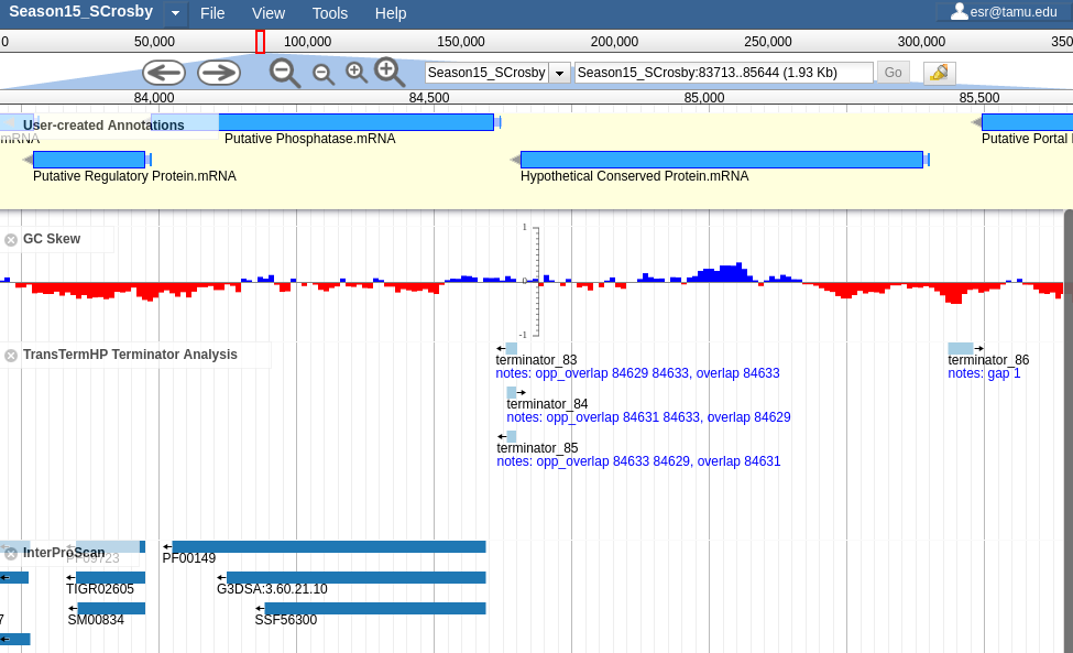
Fig. 2.1 Screenshot of Apollo with a number of different analysis tracks visisble.
2.1. Background
Apollo is a Genome Browser. It lets you visualize evidence from analyses on a genome, create and edit genes, and create and edit annotations on those genes.
Genome Browsers are a vital tool for rapidly annotating genomes. They let you visualize multiple data sources and help you synthesize those into a rational set of annotations.
2.1.1. Definitions
This portion of the course requires you to use computer resources. There are a couple of terms we use that you may or may not be familiar with, specifically in the context of software development and operations.
- Static
- Unmodifiable. Specifically in the context of a computer resource that you are accessing. The website that you see cannot be modified by you, the user accessing them. This is opposed to “dynamic” where you can interact with the files or service, and your interactions can persist.
- Instance
- A specific copy of a web service made available over the internet. Given that the administrators can run 0-N copies of the same web service, we use the term “instance” to refer to a specific copy of a service.
- Tracks
- A set of analysis results that can be shown or hidden depending on the annotator’s needs.
- Feature
- Conceptually, a region of a genome with some annotations (such as a Name, Product, or Dbxref). Visually, a rectangular box in a track.
- Evidence
- Tracks contain evidence; these are results of specific computer methods (which are documented and citable), which we use to make annotations. Annotations should not be made without evidence. Evidence allows us to move the annotation process from an art to a science.
- Annotations
- Annotation is the addition of descriptive features to a DNA sequence, such as a protein’s function, or locating tRNAs, and terminators. The annotation process we do is 100% computer based, so keep in mind that until an annotation is experimentally tested in the lab, it is putative or assumed based on an educated hypothesis.
2.1.2. GMOD, GBrowse, JBrowse, and Apollo
This section will cover a bit of history about Genome Browsers. While not useful to the annotation process, it is important to know what the terms mean and how the parts all fit together, so that the developers and annotators can have a common language.
We use a lot of software under the umbrella term of GMOD, the Generic Model Organism Database.
GMOD is a collection open source software for maintaining Model Organism Databases (MODs). Having a common platform for MODs is important, as historically individual labs spent effort building their own, custom organism databases, and then faced challenges trying to interoperate with other databases. With GMOD and the associated tools, software that talks to one MOD can be re-used when talking to another MOD. We can use the same tools to work with the CPT’s Phage Database, as people use to access data in Yeast genome databases.
2.1.2.1. Artemis
The first genome browser we will talk about is not actually a GMOD project. Artemis was an older, desktop-based genome browser. You had to install the software on your computer in order to run it. All of the other genome browsers we will look at today are web-based.
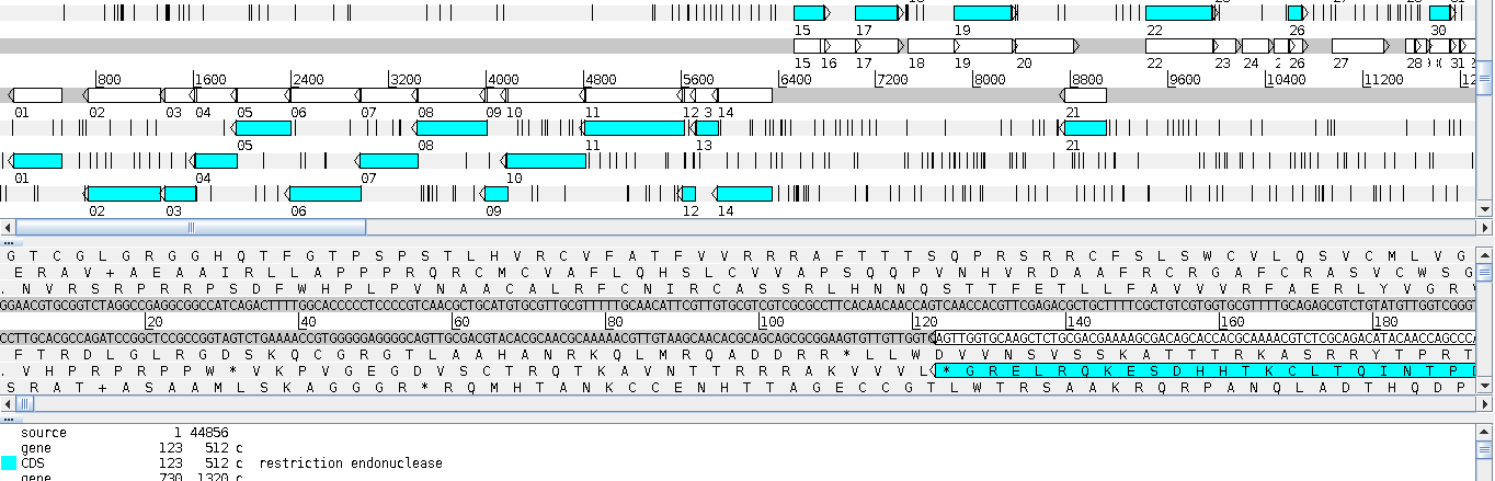
Fig. 2.2 Artemis featured a three-pane view. The panes consisted of a high-level overview of the genome, a dna-level view, and then a list of all the features in the genome.
Artemis allowed for annotation, but those annotations were only stored on your computer.
2.1.2.2. GBrowse
GBrowse was one of the earlier genome browsers. GBrowse did not support annotation.
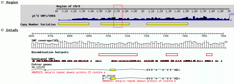
Fig. 2.3 Screenshot of GBrowse from GMOD Wiki
Think of it like the old Yahoo-maps. Instead of just clicking and dragging the map, you had to click where you wanted to go, wait a few seconds, and the new map would be displayed. It makes the process tedious.
2.1.2.3. JBrowse
We use JBrowse in our workflows for genome visualization. JBrowse is a more modern re-implementation of GBrowse. JBrowse is much more like Google Maps (or any other current web map service). You click and drag and can quickly browse around the genome, turning evidence tracks on and off where relevant.
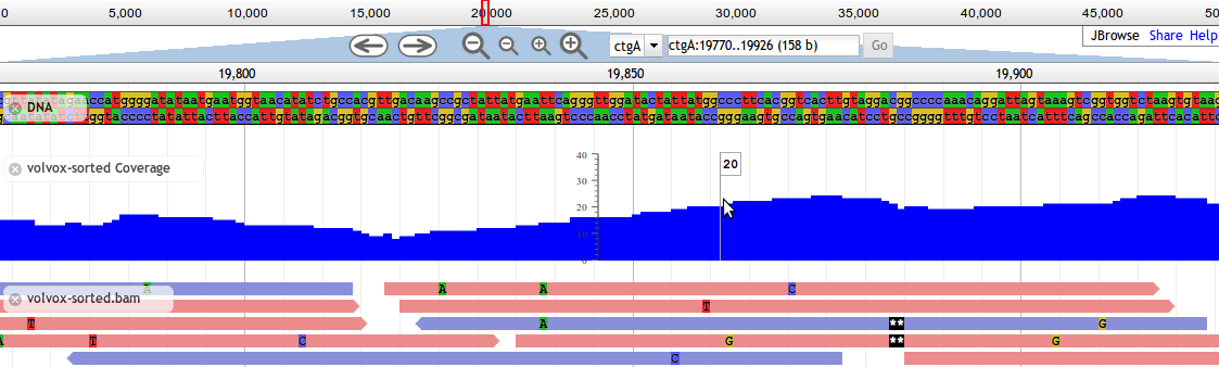
Fig. 2.4 Screnshot of a JBrowse instance. In this figure, JBrowse is shown displaying some alignments of sequencing reads to a genome.
Many labs have deployed JBrowse instances to help showcase their annotation efforts to the community, and to make their data accessible. FlyBase has produced a demo in JBrowse, displaying Drosophila melanogaster.
Note that JBrowse is a static visualization tool. You cannot make any changes to the data, and you cannot make annotations and save them. It is a “Read Only” view of genomes and annotations.
2.1.2.4. Apollo
Apollo takes JBrowse one step further and adds support for community annotation; it provides a “Read+Write” view of genomes. You can create new annotations on new gene features, and these are shared with everyone who has access to the Apollo server.
From a computer perspective, Apollo embeds a copy of JBrowse. For the annotation workflow, we will use both Apollo and JBrowse. You can see a picture of apollo in apollo-png
2.1.2.5. Summary
| Software | Availability | Allows Annotation | Notes |
|---|---|---|---|
| Artemis | Desktop Only | Yes | Used to use this; we no longer do for course purposes |
| GBrowse | Web Only | No | |
| JBrowse | Web and Desktop | No | Used for visualization of complex analyses where annotation is not required. |
| Apollo | Web Only | Yes | An additional layer on top of JBrowse to allow for annotation |
2.1.3. Annotation File Formats
There are two formats you need to be aware of during genome annotation.
- Fasta: stores genomic sequence information
- GFF3: stores genome annotations
- GenBank: an older format containing annotations and sequence information
2.1.3.1. Fasta
This is an example of fasta data:
>phiX Complete genome sequence of phage X
ACTGACTGATCGACTGCGTACGATCGACTGACTCTGCGTACGATCGACTGACTACTGACTGATCGA
TGATCGACTGCGTACGATCGACTGACTCTGCGTACGATCGACTGACTACTGACTGATCGAACTGAC
...
- Each sequence starts with a
>, - After the
>is the “fasta ID” - Some sequences have a “description” after any whitespace character, like the in the above “Complete genome...”
The sequences contained within a fasta file may be DNA, RNA, or protein
sequences. They may contain unspecified bases, N/Y/X, or - (gaps).
2.1.3.2. GFF3
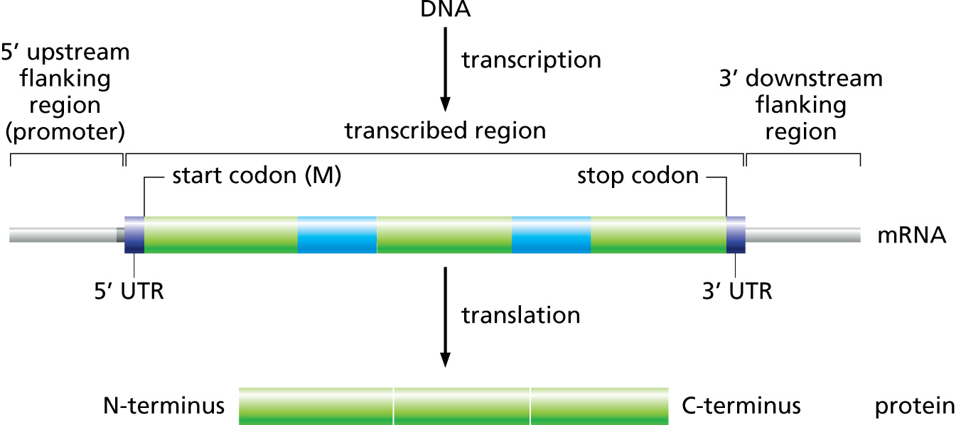
Fig. 2.5 This model is not used by phages, but is used by the storage format that all of our data is stored in.
Many of you are probably familiar with the eukaryotic gene model. This model captures a lot of information about the biological process behind producing proteins from DNA, such as mRNAs, transcription, and alternative splicing. GFF3 files thus have to encode these complex, hierarchical, parent-child relationships.
Let’s look at what a GFF3 file looks like:
##gff-version 3.2.1
##sequence-region   ctg123 1 1497228
ctg123 . gene            1000  9000  .  +  .  ID=gene00001;Name=EDEN

ctg123 . mRNA            1050  9000  .  +  .  ID=mRNA00001;Parent=gene00001;Name=EDEN.1

ctg123 . exon            1201  1500  .  +  .  ID=exon00002;Parent=mRNA00001
ctg123 . exon            3000  3902  .  +  .  ID=exon00003;Parent=mRNA00001
ctg123 . exon            5000  5500  .  +  .  ID=exon00004;Parent=mRNA00001
ctg123 . exon            7000  9000  .  +  .  ID=exon00005;Parent=mRNA00001

ctg123 . CDS             1201  1500  .  +  0  ID=cds00001;Parent=mRNA00001;Name=edenprotein.1
ctg123 . CDS             3000  3902  .  +  0  ID=cds00001;Parent=mRNA00001;Name=edenprotein.1
ctg123 . CDS             5000  5500  .  +  0  ID=cds00001;Parent=mRNA00001;Name=edenprotein.1
ctg123 . CDS             7000  7600  .  +  0  ID=cds00001;Parent=mRNA00001;Name=edenprotein.1
And the visual representation of the above text
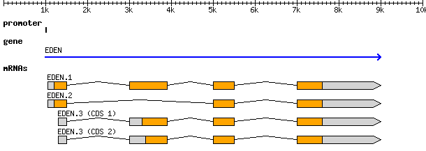
At the top level we see a “gene” (3rd column), which spans from 1000 to
9000, on the forward strand (7th column), with an ID of gene00001
and a Name of EDEN.
“Below” the gene is an mRNA feature. The mRNA has
a Parent attribute (Parent=gene00001) set to the ID of the “parent” gene
feature. This makes it a child of the gene feature.
Similarly all four exons and all four CDSs have a Parent of mRNA00001.
ID, Name, and Parent are all known as feature attributes,
metadata about a feature. Feature attributes also contain other fields; you
will see sometimes see Notes, Products, and many others. Only a handful of these
attributes have standards defining what information they contain, and the rest are
free to be used as you like. From a computational perspective, we prefer the
fields with standardised meanings. If they conform to a standard, we can apply
automation in our processing. If they are a free-form “notes” field, we need a
human to interpret and codify the evidence.
All of this is a little bit excessive for phages (where exons are rare, and mRNAs not involved), but nevertheless, we want to make sure our data is accessible to other researchers so they can do experiments building on our work. Part of this requires that we conform to standard formats and conventions used by other groups.
(It is more important that you know the format exists and that it encodes parent-child biological relationships, than the precise specifics of what each column means.)
2.1.3.3. GenBank
In stark contrast to the simplicity of the GFF3 format (tab separated, key-value pairs that are easy to work with), there is the older GenBank format. This is a fixed-width format which has a “flat” gene model, and lacks any way to represent the hierarchical relationships that are biologically relevant.
There are a few major regions of a GenBank file:
- The header (Starting with LOCUS...)
- The feature table (Starting with FEATURES)
- The sequence
The header will tell you information like:
- Sequence ID (NC_001133 in the above example)
- Genome or chromosome length
- Annotation set version (9, from
VERSION NC_001133.9) - References
LOCUS       NC_001133             230218 bp    DNA     linear   PLN 14-JUL-2011
DEFINITION  Saccharomyces cerevisiae S288c chromosome I, complete sequence.
ACCESSION   NC_001133
VERSION     NC_001133.9  GI:330443391
DBLINK      Project: 128
KEYWORDS    .
SOURCE      Saccharomyces cerevisiae S288c
  ORGANISM  Saccharomyces cerevisiae S288c
            Eukaryota; Fungi; Dikarya; Ascomycota; Saccharomycotina;
            Saccharomycetes; Saccharomycetales; Saccharomycetaceae;
            Saccharomyces.
REFERENCE   1  (bases 1 to 230218)
  AUTHORS   Goffeau,A., Barrell,B.G., Bussey,H., Davis,R.W., Dujon,B.,
            Feldmann,H., Galibert,F., Hoheisel,J.D., Jacq,C., Johnston,M.,
            Louis,E.J., Mewes,H.W., Murakami,Y., Philippsen,P., Tettelin,H. and
            Oliver,S.G.
  TITLE     Life with 6000 genes
  JOURNAL   Science 274 (5287), 546 (1996)
   PUBMED   8849441
The feature table usually starts with a “source” type feature, which
contains information about the chromosome or genome. Features consist of a
feature type key on the left, and key-value pairs on the right formatted
as /key="Value...".
FEATURES             Location/Qualifiers
     source          1..230218
                     /organism="Saccharomyces cerevisiae S288c"
                     /mol_type="genomic DNA"
                     /strain="S288c"
                     /db_xref="taxon:559292"
                     /chromosome="I"
     gene            complement(1807..2169)
                     /gene="PAU8"
                     /locus_tag="YAL068C"
                     /db_xref="GeneID:851229"
     mRNA            complement(<1807..>2169)
                     /gene="PAU8"
                     /locus_tag="YAL068C"
                     /transcript_id="NM_001180043.1"
                     /db_xref="GI:296142466"
                     /db_xref="GeneID:851229"
     CDS             complement(1807..2169)
                     /gene="PAU8"
                     /locus_tag="YAL068C"
                     /note="hypothetical protein, member of the seripauperin
                     multigene family encoded mainly in subtelomeric regions"
                     /codon_start=1
                     /protein_id="NP_009332.1"
                     /db_xref="GI:6319249"
                     /db_xref="SGD:S000002142"
                     /db_xref="GeneID:851229"
...
Lastly, there is the sequence data. GenBank shows the sequence separated into six columns of ten characters, with the sequence index annotated on the left.
ORIGIN
        1 ccacaccaca cccacacacc cacacaccac accacacacc acaccacacc cacacacaca
       61 catcctaaca ctaccctaac acagccctaa tctaaccctg gccaacctgt ctctcaactt
2.2. Annotation
On to actually using Apollo! We’ll go through an example annotation. You’re welcome to follow along with this at home and familiarize yourself with Apollo before class. The example presented here will be open for everyone in the class to use, so images may not reflect the current annotations made.
Warning
As of 2016-02, the Apollo service does NOT work under IE11.
There are two primary components to annotation:
- Structural annotation
- Functional annotation
In structural annotation, several gene callers will identify possible genes in your phage genome. You will annotate putative genes in Apollo based on these results. Structural annotations consist of locations of genomic features, like genes and terminators.
Functional annotation entails identifying possible gene functions based on multiple sources of evidence.
We will go into more detail in the first lecture on what it means to do structural and functional annotations.
2.2.1. Apollo in Galaxy
This section will cover the generalised use of Apollo in Galaxy, nonspecific to any workflow implementation.
2.2.1.1. JBrowse In Galaxy
The CPT developed a tool called JBrowse-in-Galaxy (JiG), which allows you to build JBrowse instances within Galaxy. This contrasts with how JBrowse instances are traditionally configured, through a complex and manual process at the command line.
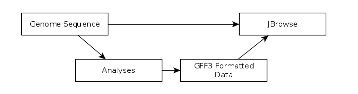
Fig. 2.6 The generalized JBrowse workflow. We use JBrowse as a tool for displaying the results of a bioinformatic analysis in a standardised way. Instead of having to digest and understand 20+ different report formats, images, output files, tables, etc., all of our analysis is presented as easy-to-grasp features in evidence tracks.
Apollo takes, as its input, complete JBrowse instances. To view any data in Apollo, a JBrowse instance needs to be configured first.
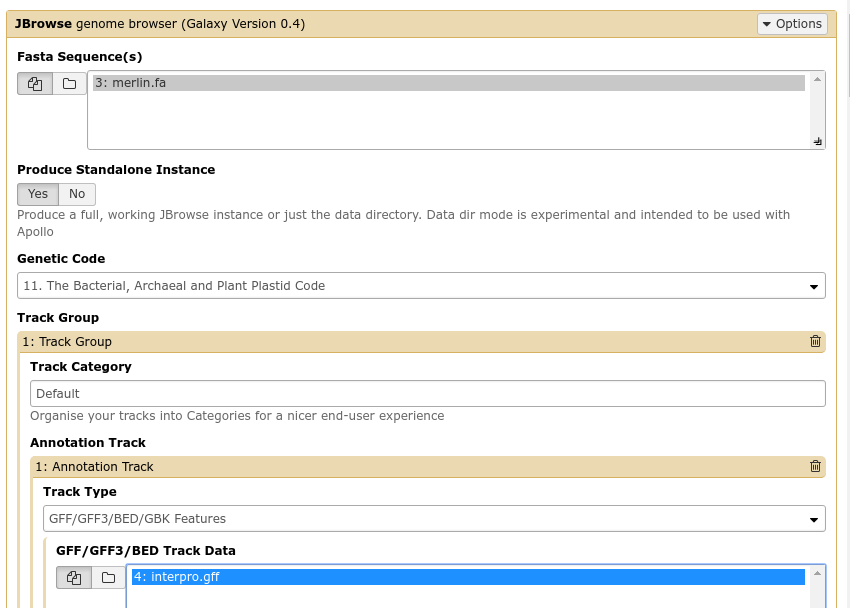
Fig. 2.7 The JBrowse-in-Galaxy tool is an extremely complex tool, with a very detailed manual (at the bottom of the page in Galaxy). If you need to do anything beyond showing simple GFF3 files, you’ll need to read this manual.
Once you’ve created a JBrowse instance, you will find it in your history. You can click the eyeball to see the JBrowse instance in the main panel, or you can click the floppy disk to save the JBrowse instance to your computer (but generally there is no need to do this, as it will always be available in your Galaxy history.)
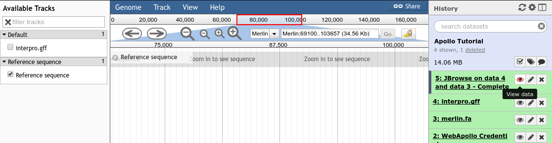
Fig. 2.8 Viewing a JBrowse instance produced within Galaxy.
2.2.1.2. Moving Data from Galaxy to Apollo
Now that you have a complete JBrowse instance, you’re ready to start talking to the Apollo service.
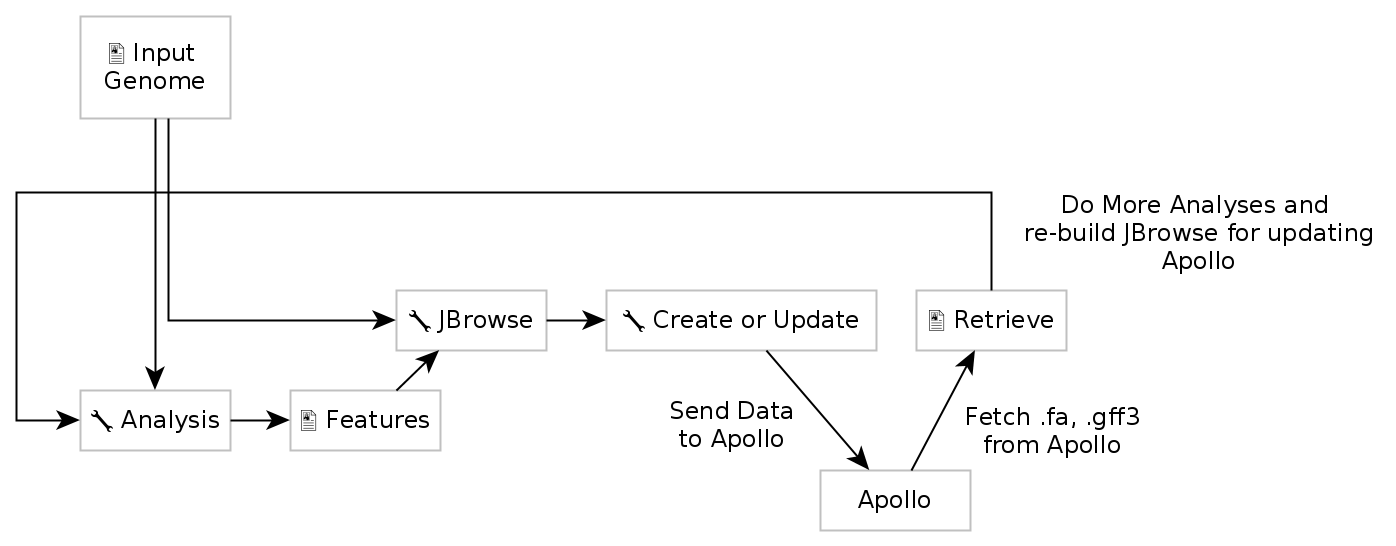
Fig. 2.9 The general Apollo/JBrowse-in-Galaxy/Galaxy workflow. Data is built up in Galaxy in the form of a JBrowse instance, which is pushed to the Apollo service in the Create or Update step. Once annotations are made, we can export the updated set of annotations from Apollo into Galaxy, and then re-analyse and update Apollo with new results.
The first tool we’ll use is a tool named Create or Update, which lets us create, or update, an organism in Apollo with new data from Galaxy in the form of a JBrowse instance.
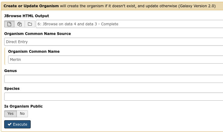
Fig. 2.10 You must fill out the Organism Common Name. If your phage is “Petty”, it is
recommend that 1) your fasta file header reads >Petty (and nothing
else), and that 2) you write “Petty” in the Common name field here.
This step will transfer data to Apollo, and produce a JSON file. The output JSON file contains some metadata about the organism.
With your data available in Apollo, you can access it at Apollo (NB: you must be logged in to Galaxy to access Apollo), or via the Annotate convenience tool. The Annotate tool takes the JSON file from a Create or Update step, and loads Apollo, directly in Galaxy.
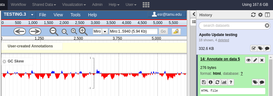
Fig. 2.11 Apollo accessed from within Galaxy
2.2.2. Finding Our Way Around
In Apollo, you’ll be presented with a two-pane display. On the left is an embedded JBrowse instance. On the right is the Apollo annotator panel.
JBrowse, embedded in Apollo, is slightly different than a normal JBrowse. The movement controls are all the same:
- you can use the magnifying glasses to zoom in and out of the genome and its data
- the arrow icons will move you up and downstream along the genome
- Selecting or clicking on locations along the genome ruler (the light grey box at the top of the genome, 0 bp; 20,000bp; 40,000bp; etc.) will allow you to zoom in and move to specific regions
The menu bar has some useful options, some that aren’t available in “standard” JBrowse:
- View will let you set some useful options:
- “Color by CDS frame” is a popular option during annotation. It will colour each coding sequence by which frame the reading frame is in.
- “Show Track Label” is an incredibly useful feature to hide the track’s labelling, allowing you to annotate small features near the end of the genome, which would otherwise be hidden by the track label (E.g. “User created annotations”)
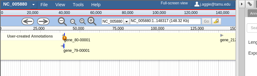
The pale yellow track that is visible is the User Created Annotation track. During the annotation of a genome, gene features will be added to this track and edited, thus this track will always be visible to you.
On the right is the Genome Selector, which lists all of the organisms accessible to you.
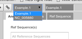
Fig. 2.12 Organism selection menu
Apollo uses the concept of “Organisms” with “reference sequences” below it. Each organism can have one or more reference sequences. In higher order organisms, those often correspond to multiple chromosomes. For phage uses they are most often used to correspond to different assemblies of the genome. We will only work with organisms with a single reference sequence in this class.
Just as in JBrowse, the “Track List” is on the left. If you select the gene call tracks (GeneMarkS, MetaGeneAnnotator, and Glimmer3), they will show up in JBrowse. You may find that this produces an absolutely overwhelming amount of information:
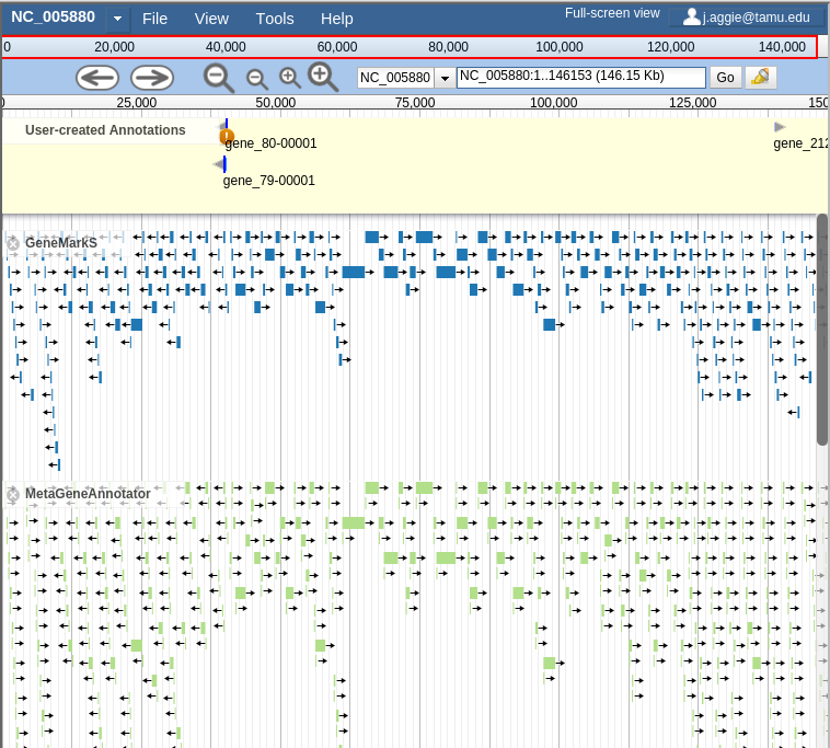
Fig. 2.13 Overwhelming
In order to combat that, you should zoom in:
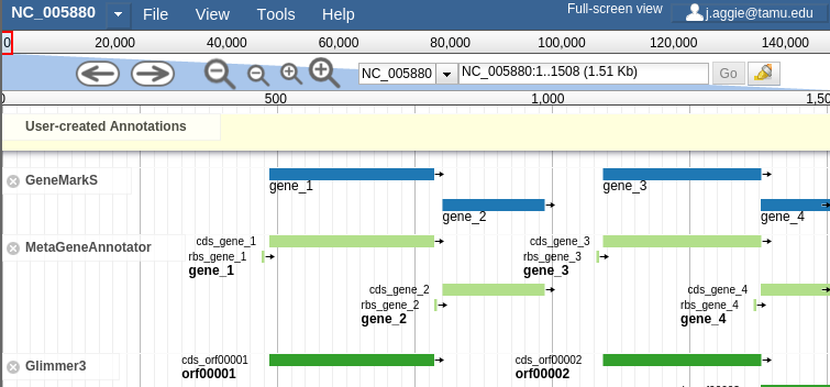
Fig. 2.14 Zooming
You may find that you wish to focus solely on the annotation process, without any distractions from the Apollo portion of the interface. You can hide that easily.
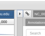
Fig. 2.15 Hiding Apollo
Let’s zoom down to the level of a single gene:
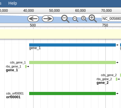
Fig. 2.16 Here we can begin to compare the gene models of these three genes. One of the three has a Shine Dalgarno sequence anotated. The CPT filters all SD sequences to ensure that only high quality ones are visible.
Great! Here we see the very first gene called by the three gene callers that we use. (There is more information on gene calling available in the Pipeline document. We will cover that separately. A gene call is a possible location for a gene)
Note
Just like Galaxy, your work is saved automatically and instantaneously. You do not need to worry about losing changes.
2.2.3. Deleting Features
If you find that you create a feature you did not want, you can delete it by double-clicking the feature and then selecting “Delete Feature”. If you do not double click, it might not delete properly.
2.3. Workflows
There are a couple of workflows which you will run as part of the Apollo and Annotation process. The first covers structural annotation (genes, terminators, tRNAs), while the second covers functional annotation (blast, interpro, etc.).
2.3.1. Starting
If you have your phage’s genome, then you’re reading to start with Structural Annotation Workflow
